Three-point bending test

The first example is concerned with simple two-dimensional analysis of a simply supported concrete beam loaded by a concentrated force (Fig. 1a). Due to symmetry, the centerline of the process zone is straight and the failure mechanism corresponds to pure Mode-I fracture. The constitutive properties are set to: Young's modulus $E=20$ GPa, Poisson's ratio $\nu=0.2$, tensile strength $f_t=2$ MPa, strain controling the softening $\varepsilon _f=0.002$, and nonlocal interaction radius $R=20$ mm. The mesh contains 696 nodes and 1298 constant-strain elements (Fig. 1b).

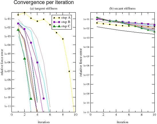
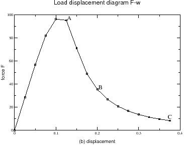
The formation of the process zone and failure of the specimen are simulated in 15 incremental steps, controled by imposed increments of the displacement under the applied load. The load-displacement diagram is shown in Fig. 3. Three solution strategies are compared:

• SSM-10: secant stiffness matrix updated after each 10 equilibrium iterations.
• SSM-5: secant stiffness matrix updated after each 5 equilibrium iterations.
• TSM: fully consistent nonlocal tangent stiffness matrix updated after each equilibrium iteration.

The rates of convergence of the global equilibrium iteration procedure are illustrated in Fig. 2, which shows the dependence of the error (norm of residual forces) on the number of iterations. As expected, the secant stiffness leads only to a linear convergence rate, i.e., the logarithm of the error $r_n$ is approximately a linear function of the iteration number, $n$. With increasing $n$, the ratio $r_{n+1}/r_n$ tends to $\exp(c)$ where $c<0$ is the slope of the straight line in the semilogarithmic convergence plot in Fig. 2b. The steps A, B and C correspond to peak, post-peak and fully damaged regime, as indicated in the load-displacement diagram in Fig. 3.

For the tangent stiffness, the convergence rate is quadratic, i.e., the convergence curves are approximately parabolic (Fig. 2a). The residual is then reduced to the level of machine precision within a few iterations, typically 3 to 6. The only exception is step 5 (around the peak of the load-displacement curve), in which the initial prediction is not sufficiently close to the exact solution, and the quadratic rate of convergence is attained only after iteration number 7.

Figure 1: Three-point bending test: (a) specimen geometry and loading, (b) finite element mesh

Figure 2: Three-point bending test: convergence characteristics

Figure 3: Three-point bending test: load displacement diagram

The relative efficiency of the strategies using the secant or tangent stiffness matrices strongly depends on the prescribed convergence tolerance. For a relative tolerance $\epsilon=10^{-3}$, the number of iterations per step using SSM-10 does not exceed 68; see Table 1. With TSM, the number of iterations per step is at most 8, but each iteration is much more costly. The secant stiffness matrix is symmetric and has a smaller average bandwidth than the nonsymmetric tangent stiffness matrix. Moreover, the rate of convergence is not substantially reduced if the secant stiffness is assembled and factorized only once per every 10 iterations, which results into additional savings. The tangent stiffness must be updated in every iteration, otherwise the quadratic rate of convergence would be lost. As shown in Table 2, the total time needed for the complete analysis using SSM-10 is more than three times shorter than that needed by TSM with a direct solver. For this small problem, an iterative solver would not be advantageous. The assembly procedure takes 0.02 seconds for SSM-10 approach, while for TSM approach it takes between 0.02 to 1.2 seconds. The factorization time for SSM-10 approach is constant, equal to 0.34 seconds, while for TSM approach it varies between 0.75 and 1.06 seconds.

The relative efficiency of SSM and TSM changes dramatically if a strict convergence criterion is required. For a relative tolerance $\epsilon=10^{-6}$, the number of iterations per step using SSM-10 becomes excessive, and no improvement is obtained if the stiffness matrix is updated after every 5 iterations; see Table 3. On the other hand, TSM typically converges within 3 to 6 iterations, and only in one step it needs 10 iterations. As a result, the total analysis with TSM is now more than 3 times faster than with SSM-10; see Table 2.

Table 1: Three-point bending test: convergence and times per iteration (``nite'' is the number of equilibrium iterations) for tolerance $\epsilon=10^{-3}$

	SSM-10		TSM
step	nite	time[s]	nite	time[s]
1	1	0.30	1	0.60
2	1	0.30	1	0.60
3	14	1.61	3	3.66
4	34	3.65	3	6.94
5	46	4.78	8	17.35
6	36	3.75	4	10.45
7	27	2.78	4	11.30
8	23	2.42	3	9.37
9	29	2.93	4	12.01
10	63	6.25	3	9.82
11	68	6.75	2	7.53
12	55	5.55	2	7.62
13	46	4.57	2	7.64
14	19	1.96	2	7.74
15	15	1.62	2	7.69

Table 2: Three-point bending test: total analysis times for different strategies and different convergence tolerances

tolerance	strategy	total time
$\epsilon=10^{-3}$	SSM-10	00m:50s
	TSM	02m:01s
$\epsilon=10^{-6}$	SSM-10	14m:33s
	SSM-5	15m:03s
	TSM	03m:52s

Table 3: Three-point bending test: convergence and times per iteration (``nite'' is the number of equilibrium iterations) for tolerance $\epsilon=10^{-6}$

	SSM-10		SSM-5		TSM
step	nite	time[s]	nite	time[s]	nite	time[s]
1	1	0.32	1	0.32	1	0.60
2	1	0.32	1	0.32	1	0.60
3	46	4.98	44	4.82	4	4.73
4	110	11.38	108	11.63	4	8.81
5	191	19.11	187	19.27	10	21.45
6	426	41.79	423	42.90	6	14.85
7	696	67.34	694	69.91	6	15.91
8	807	77.91	805	80.28	5	14.21
9	732	70.49	730	72.68	6	16.85
10	813	77.86	811	80.84	5	14.69
11	897	85.79	895	88.55	4	12.58
12	989	94.26	986	97.84	4	12.97
13	1053	98.27	1051	104.07	4	12.87
14	1153	110.18	1151	113.60	3	10.33
15	1156	112.30	1155	115.68	3	10.43

This example indicates that for a low accuracy the strategy using a secant stiffness matrix is numerically more efficient. For a high accuracy, the results illustrate the potential benefits of the tangent stiffness matrix. The overhead of storing the whole matrix instead of its symmetric part and of the more time-consuming solution procedure is more than compensated by very fast convergence.