Elements

In this frame, the following base classes are introduced:

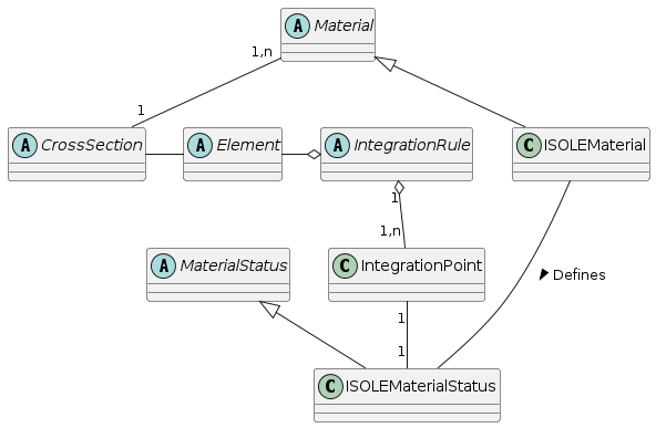
• Class Element, which is an abstraction of a finite element. It declares common general services, provided by all elements. Derived classes are the base classes for specific analysis types (structural analysis, thermal analysis). They declare and implement necessary services for specific analysis.

• Class IntegrationPoint is an abstraction for the integration point of the finite element. For historical reasons the IntegrationPoint is an alias to GaussPoint class. It maintains its coordinates and integration weight. Any integration point can generally contain any number of other integration points - called slaves. The IntegrationPoint instance containing slaves is called master. Slaves are, for example, introduced by a layered cross section model, where they represent integration points for each layer, or can be introduced at material model level, where they may represent, for example, micro-planes. Slave integration points are hidden from elements. The IntegrationPoint contains associated material status to store state variables (the reasons for introducing this feature will be explained later).

• CrossSection class is an abstraction for cross section. Its main role is to hide from an element all details concerning the cross section description and implementation. By cross section description is meant, for example, an integral cross section model, layered cross section model or fibered model. Elements do not communicate directly with material, instead they always use a CrossSection, which performs all necessary integration over its volume and invokes necessary material class services. Note, that for some problems, the use of cross section is not necessary, and then the elements can communicate directly with material model. However, for some problems (for example structural analysis) the introduction of cross section is natural.

• Material class is the base class for all constitutive models. Derived classes should be the base analysis-specific classes, which declare required analysis specific services (for example structural material class declares services for the stiffness computation and services for the real stress evaluation). Similarly to cross section representation, the material model analysis specific interface, defined in terms of general services, allows the use of any material model, even that added in the future, without modifying any code, because all material models implement the same interface.

One of the most important goals of OOFEM is its extensibility. In the case of extension of the material library, the analyst is facing a key problem. Every material model must store its unique state variables in every integration point. The amount, type, and meaning of these history variables vary for each material model. Therefore, it is not possible to efficiently match all needs and to reflect them in the integration point data structure. The suggested remedy is the following:

The IntegrationPoint class is equipped with the possibility to have associated a MaterialStatus class instance. When a new material model is implemented, the analyst has also to declare and implement a related material status derived from the base MaterialStatus class. This status contains all necessary state variables and related data access and modification services. The IntegrationPoint provides services for inserting and accessing its related status. For every IntegrationPoint, the corresponding material creates unique copy of its material status and associates it with that integration point. Because the IntegrationPoint is a compulsory parameter of all Material class methods, the state variables are always accessible.

OOFEM Top level structure

In Fig (fig-elementmaterialframe), the material - element frame is depicted in more detail, although still simplified.

Element class

This class is the base class for all FE elements. It is also the abstract class, declaring some services, which have to be implemented by the derived classes. The main purpose of this class is to define a common interface and attributes, provided by all individual element implementations. The Element` class does neither declare nor implement any method related to specific analysis. These services are to be declared and possibly implemented by derived classes. The direct child of Element class are assumed to be the base classes for particular analysis or problem type. They typically introduce the general services required for a specific analysis purpose - like evaluation of stiffness or mass matrices for structural analysis, or evaluation of capacity and conductivity matrices for heat transfer analysis. Usually they also provide generic implementation of these services.

The Element class is derived from parent FEMComponent, leke many other classes. It inherits the FEMComponent ability to keep its number and reference to the domain, it belongs to, its error and warning reporting services. Also the FEMComponent class introduces several abstract services. The most important are

• initializeFrom for object initialization from a given record,

• saveContext and restoreContext methods for storing and restoring object state to/from a stream

The attributes defined by the Element class include the arrays used to keep its list of nodes and sides, variables to store its material and cross section number, lists of applied body and boundary loads, list of integration rules and array storing its code numbers.

The following important services are declared/introduced by the Element:

• services for component management - include services for accesing element’s nodes, material and cross section (giveDofManager, giveNode, giveNumberOfDofManagers, giveNumberOfNodes, giveMaterial, giveCrossSection).

• services related to code numbers management:

  • giveLocationArray returns the element location array. This location array is obtained by appending code-numbers of element nodes (according to the node numbering), followed by code numbers of element sides. The ordering of DOFs for the particular node/side is specified using a node/side DOF mask, which is obtained/defined by giveNodeDofIDMask or giveSideDofIDMask services. Please note, that this local DOF ordering must be taken into account when assembling various local characteristic vectors and matrices. Once the element location array is assembled, it is cached and reused to avoid time consuming assembly. Some engineering models may support dynamic changes of the static system (generally, of boundary conditions) during analysis, then these models use invalidateLocationArray function to invalidate location array after finishing time step, to force new equation numbering.

  • computeNumberOfDofs - computes or simply returns total number of element’s local DOFs. Must be implemented by particular element.

  • giveDofManDofIDMask service return DOF mask for corresponding dof manager (node or side). This mask defines the DOFs which are used by element at the given node/side. The mask influences the code number ordering for the particular node. Code numbers are ordered according to the node order and DOFs belonging to the particular node are ordered according to this mask. If element requests DOFs using a node mask which are not in the node then error is generated. This masking allows node to be shared by different elements with different DOFs in the same node/side. Element’s local code numbers are extracted from the node/side using this mask. These services must be implemented (overloaded) by particular element implementations.

• services for requesting the so-called characteristic components: giveCharacteristicMatrix and giveCharacteristicVector. The component requested is identified by parameter of type CharType (see cltypes.h). These are general methods for obtaining various element contributions to the global problem. These member functions have to be overloaded by derived analysis-specific classes in order to invoke the proper method according to the type of requested component.

• services related to the solution step update and termination. These services are used to update the internal variables at element’s integration points prior to reached state updateYourself and updateInternalState. Similar service for the internal state initialization is also declared (initializeYourself) and re-initialization to previous equilibrium state (see initForNewStep).

• services for accessing local element’s unknowns from corresponding DOFs. These include methods for requesting local element vector of unknowns (computeVectorOf) and local element vector of prescribed unknowns (computeVectorOfPrescribed).

• Services for handling transformations between element local coordinate system and coordinate system used in nodes (possibly different from global coordinate system).

• Othetr miscellaneous services. Their detailed description can be found in Element class definition in src/core/element.h.

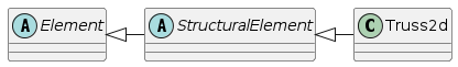
Analysis specific element classes

The direct child classes of the Element class are supposed to be (but not need to be) base classes for particular problem types. For example, the StructuralElement class is the base class for all structural elements. It declares all necessary services required by structural analysis (for example methods computing stiffness matrices, load, strain and stress vectors etc.). This class may provide general implementations of some of these services if possible, implemented using some low-level virtual functions (like computing element shape functions), which are declared, but their implementation is left on derived classes, which implement specific elements.

Structural element

To proceed, lets take StructuralElement class as an example. This class is derived from the Element class. The basic tasks of the structural element is to compute its contributions to global equilibrium equations (mass and stiffness matrices, various load vectors (due to boundary conditions, force loading, thermal loading, etc.) and computing the corresponding strains and stresses from nodal displacements. Therefore the corresponding virtual services for computing these contributions are declared. These standard contributions can be computed by numerical integration of appropriate terms, which typically depend on element interpolation or material model, over the element volume. Therefore, it is possible to provide general implementations of these services, provided that the corresponding methods for computing interpolation dependent terms and material terms are implemented, and corresponding integration rules are initialized.

This concept will be demonstrated on service computing stiffness matrix. Since element stiffness matrix contributes to the global equilibrium, the stiffness will be requested (by engineering model) using giveCharacteristicMatrix service.

void
StructuralElement ::  giveCharacteristicMatrix (FloatMatrix& answer,
                    CharType mtrx, TimeStep *tStep)
//
// returns characteristic matrix of receiver according to mtrx
//
{
if (mtrx == TangentStiffnessMatrix)
    this -> computeStiffnessMatrix(answer, TangentStiffness, tStep);
else if (mtrx == SecantStiffnessMatrix)
    this -> computeStiffnessMatrix(answer, SecantStiffness, tStep);
else if (mtrx == MassMatrix)
    this -> computeMassMatrix(answer, tStep);
else if
....
}

The first parameter is the matrix to be computed, the mtrx parameter determines the type of contribution and the last parameter, time step, represents solution step. Focusing only on material nonlinearity, the element stiffness matrix can be evaluated using well-known formula

\[{K} = \int_{V} {B}^T{D}{B}\;dV,\]

where B is the so-called geometrical matrix, containing derivatives of shape functions and D is the material stiffness matrix. If D is symmetric (which is usually the case) then element stiffness is symmetric, too. The numerical integration is used to evaluate the integral. For numerical integration, we will use IntegrationRule class instance. The integration rules for a specific element are created during element initialization and are stored in integrationRulesArray attribute, defined/introduced by the parent Element class. In order to implement the stiffness evaluation, the methods for computing geometrical matrix B and material stiffness matrix D are declared (as virtual), but not implemented. They have to be implemented by specific elements, because they know their interpolation and material mode details. The implementation of computeStiffnessMatrix` is as follows:

void
StructuralElement :: computeStiffnessMatrix (FloatMatrix& answer,
                    MatResponseMode rMode, TimeStep* tStep)
// Computes numerically the stiffness matrix of the receiver.
{
int j;
double      dV ;
FloatMatrix d, bj, dbj;
GaussPoint  *gp ;
IntegrationRule* iRule;

// give reference to integration rule
iRule = integrationRulesArray[giveDefaultIntegrationRule()];

// loop over integration points
for (j=0 ; j < iRule->getNumberOfIntegrationPoints() ; j++) {
    gp = iRule->getIntegrationPoint(j) ;
    // compute geometrical matrix of particular element
    this -> computeBmatrixAt(gp, bj) ;
    //compute material stiffness
    this -> computeConstitutiveMatrixAt(d, rMode, gp, tStep);
    // compute jacobian
    dV = this -> computeVolumeAround(gp) ;
    // evaluate stiffness
    dbj.beProductOf (d, bj) ;
    answer.plusProductSymmUpper(bj,dbj,dV) ;
}
answer.symmetrized() ;
return  ;
}

Inside the integration loop, only the upper half of the element stiffness is computed in element local coordinate system. Then, the lower part of the stiffness is initialized from the upper part (answer.symmetrized()). The other element contributions can be computed using similar procedures. In general, different integration rules can be used for evaluation of different element contributions. For example, the support for the reduced integration of some terms of the stiffness matrix can be easily supported.

The element strain and stress vectors are to be computed using computeStrainVector and computeStressVector services. The element strain vector can be evaluated using

\[\varepsilon={B}{u},\]

where B is the geometrical matrix and u is element local displacement vector.

void
StructuralElement :: computeStrainVector (FloatArray& answer,
                    GaussPoint* gp, TimeStep* stepN)
// Computes the vector containing the strains
// at the Gauss point gp of the receiver,
// at time step stepN. The nature of these strains depends
// on the element's type.
{
FloatMatrix b;
FloatArray  u ;

this -> computeBmatrixAt(gp, b) ;
// compute vector of element's unknowns
this -> computeVectorOf(DisplacementVector,
                        UnknownMode_Total,stepN,u) ;
// transform global unknowns into element local c.s.
if (this->updateRotationMatrix())
    u.rotatedWith(this->rotationMatrix,'n') ;
answer.beProductOf (b, u) ;
return ;
}

The stress evaluation on the element level is rather simple, since the stress evaluation from a given strain increment and actual state (kept within the integration point) is done at the cross section and material model levels:

void
StructuralElement :: computeStressVector (FloatArray& answer,
                    GaussPoint* gp, TimeStep* stepN)
// Computes the vector containing the stresses
// at the Gauss point gp of the receiver, at time step stepN.
// The nature of these stresses depends on the element's type.
{
FloatArray Epsilon ;
StructuralCrossSection* cs = (StructuralCrossSection*)
                            this->giveCrossSection();
Material *mat = this->giveMaterial();

this->computeStrainVector (Epsilon, gp,stepN) ;
// ask cross section model for real stresses
// for given strain increment
cs -> giveRealStresses (answer, ReducedForm, gp, Epsilon, stepN);
return  ;
}

For further reference see src/sm/Elements/structuralelement.h and src/sm/Elements/structuralelement.C files located in your source oofem directory.

Example: 2D Truss element

In this section, we provide a simple, but complete example of a two-dimensional truss element implementation. The element is derived from the StructuralElement class and is called Truss2d:

The definition of the Truss2d class is as follows (see also sm/src/Elements/Bars/Truss2d.h):

class Truss2d : public StructuralElement {
protected :
    double        length ;
    double        pitch ;
public :
    Truss2d (int,Domain*) ;    // constructor
    ~Truss2d ()   {}           // empty destructor
    // mass matrix coputations
    void computeLumpedMassMatrix (FloatMatrix& answer,
                                 TimeStep* tStep) override;
    // general mass service overloaded
    void computeMassMatrix (FloatMatrix& answer, TimeStep* tStep) override
        {computeLumpedMassMatrix(answer, tStep);}
    // DOF management
    virtual int            computeNumberOfDofs (EquationID ut) override {return 4;}
    virtual void           giveDofManDofIDMask  (int inode, EquationID, IntArray& ) const override;

    double computeVolumeAround (GaussPoint*) override;
    // definition & identification
    char* giveClassName (char* s) const override
         { return strcpy(s,"Truss2d") ;}
    classType giveClassID () const override { return Truss2dClass; }

    IRResultType initializeFrom (InputRecord* ir) override;
protected:
    // computes geometrical matrix
    void computeBmatrixAt (GaussPoint*, FloatMatrix&,
                            int=1, int=ALL_STRAINS) override;
    // computes interpolation matrix
    void computeNmatrixAt (GaussPoint*, FloatMatrix&) override;
    // initialize element's integration rules
    void computeGaussPoints () override;
    // transformation from global->local c.s.
    int           computeGtoLRotationMatrix (FloatMatrix&) override;

    double giveLength () ;
    double givePitch () ;
} ;

The Truss2d class declares two attributes, the element length` and element pitch, defined as angle between global x-axis and element x-axis. They can be computed from coordinates of element nodes, but they are used at different places of implementation and precomputing then can save some proccesing time. We define the constructor and destructor of the Truss2d class. Next we define methods to compute characteristic contributions of the element. Note that default implementation of characteristic matrix evaluation (stiffness nad mass matrix) is already provided by parent StructuralElement class. We just need to implement the methods for computing geometrical and interpolation matrices. However in this case, the mass matrix is going to be computed using the lumped mass matrix method, and we need to overload the default implementation.

We also need to implement the methods for computing the number of element DOFs (computeNumberOfDofs), method to return element DOFs for specific node (giveDofManDofIDMask). Also, the method to evaluate the volume associated to given integration point (computeVolumeAround), method to initialize element from input record (initializeFrom). Finally, in the protected section, there is a declaration of methods for computing the geometrical ( computeBmatrixAt) and interpolation matrices (computeNmatrixAt), as well as the method to initialize the element’s integration rules (computeGaussPoints) and method to compute the element transformation matrix (computeGtoLRotationMatrix). Note than all these methods overload/specialize/define methods declared in the parent StructuralElement or Element classes. Finally, we declare two methods to compute the element length and pitch.

The implementation of the Truss2d class is as follows (see also sm/src/Elements/Bars/Truss2d.C, but note this implementation supports geometrical nonlinearity and is more general), wih some minor methods ommited for brevity: We start with the services for computing interpolation and geometrical matrices. Note that the implementation of the service{computeNmatrixAt} is not necessary for the current purpose (it would be required by the default mass matrix computation), but it is added for completeness. The both methods compute response at a given integration point, which is passed as a parameter. The service{computeBmatrixAt} has two additional parameters which determine the range of strain components for which response is assembled. This has something to do with support for reduced/selective integration and is not important in presented case.

The ordering of element unknowns is following: \(r_e=\{u1,y1, u2,y2\}^T\), where u1,u2 are displacements in x-direction and y1,y2 are displacements in y-direction and indices indicate element nodes. This ordering is defined by element node numbering and element nodal unknowns (determined by giveDofManDofIDMask method). The vector of unknowns (and also element code numbers) is appended from nodal contributions. The element uses linear interpolation functions, so the element shape functions are linear functions of the local coordinate. The element has 2 nodes, so the element has 4 DOFs. The interpolation functions are defined as follows:

\[N_1 = \frac{1-\xi}{2}, \quad N_2 = \frac{1+\xi}{2},\]

and their derivatives:

\[\frac{\partial N_1}{\partial \xi} = -\frac{1}{2}, \quad \frac{\partial N_2}{\partial \xi} = \frac{1}{2}.\]

So that the interpolation and geometrical matrices are defined as follows:

\[\begin{split}\{u,v\}^T = N^e r_e, \ \{\varepsilon\} = B^e r_e^l\\[4mm] B^e = \begin{bmatrix} -\frac{1}{L} & 0 & \frac{1}{L} & 0 \end{bmatrix},\\ \quad N^e = \begin{bmatrix} N_1 & 0 & N_2 & 0 \\ 0 & N_1 & 0 & N_2 \end{bmatrix},\end{split}\]

The transformation matrix from unknowns in global coordinate system to element local coordinate system is defined as follows:

\[\begin{split}\cos\theta = (x_2-x_1)/l,\ \sin\theta = (y_2-y_1)/l,\\[4mm] \begin{bmatrix} u_1 \\ v_1 \\ u_2 \\ v_2 \end{bmatrix}^l = \begin{bmatrix} \cos \theta & \sin \theta & 0 & 0 \\ -\sin \theta & \cos \theta & 0 & 0 \\ 0 & 0 & \cos \theta & \sin \theta \\ 0 & 0 & -\sin \theta & \cos \theta \end{bmatrix} \begin{bmatrix} u_1 \\ v_1 \\ u_2 \\ v_2 \end{bmatrix}^g,\end{split}\]

where \(\theta\) is the pitch of the element.

Note

Recently, the interpolation classes have been added, that can significantly facilitate the element implementation. They provide shape functions, their derivatives, and transformation Jacobian out of the box.

void
Truss2d ::   giveDofManDofIDMask  (int inode, EquationID, IntArray& answer) const {
// returns DofId mask array for inode element node.
// DofId mask array determines the dof ordering requested from node.
// DofId mask array contains the DofID constants (defined in cltypes.h)
// describing physical meaning of particular DOFs.
//IntArray* answer = new IntArray (2);
answer.resize (2);

answer.at(1) = D_u;
answer.at(2) = D_w;

return ;
}

void
Truss2d :: computeNmatrixAt (GaussPoint* aGaussPoint,
                            FloatMatrix& answer)
// Returns the displacement interpolation matrix {N}
// of the receiver, evaluated at aGaussPoint.
{
    double       ksi,n1,n2 ;

    ksi = aGaussPoint -> giveCoordinate(1) ;
    n1  = (1. - ksi) * 0.5 ;
    n2  = (1. + ksi) * 0.5 ;

    answer.resize (2,4);
    answer.zero();

    answer.at(1,1) = n1 ;
    answer.at(1,3) = n2 ;
    answer.at(2,2) = n1 ;
    answer.at(2,4) = n2 ;

    return  ;
}


void
Truss2d :: computeBmatrixAt (GaussPoint* aGaussPoint,
                            FloatMatrix& answer, int li, int ui)
//
// Returns linear part of geometrical
// equations of the receiver at gp.
// Returns the linear part of the B matrix
//
{
double coeff,l;

answer.resize(1,4);
l = this->giveLength();
coeff = 1.0/l;

answer.at(1,1) =-coeff;
answer.at(1,2) = 0.0;
answer.at(1,3) = coeff;
answer.at(1,4) = 0.0;

return;

Next, the following two functions compute the basic geometric characteristics of a bar element - its length and pitch, defined as the angle between global x-axis and the local element x-axis (oriented from node1 to node2).

double  Truss2d :: giveLength ()
// Returns the length of the receiver.
{
    double dx,dz ;
    Node   *nodeA,*nodeB ;

    if (length == 0.) {
    nodeA = this->giveNode(1) ;
    nodeB = this->giveNode(2) ;
    dx    = nodeB->giveCoordinate(1)-nodeA->giveCoordinate(1);
    dz    = nodeB->giveCoordinate(3)-nodeA->giveCoordinate(3);
    length= sqrt(dx*dx + dz*dz) ;}

    return length ;
}


double  Truss2d :: givePitch ()
// Returns the pitch of the receiver.
{
    double xA,xB,zA,zB ;
    Node   *nodeA,*nodeB ;

    if (pitch == 10.) {  // 10. : dummy initialization value
    nodeA  = this -> giveNode(1) ;
    nodeB  = this -> giveNode(2) ;
    xA     = nodeA->giveCoordinate(1) ;
    xB     = nodeB->giveCoordinate(1) ;
    zA     = nodeA->giveCoordinate(3) ;
    zB     = nodeB->giveCoordinate(3) ;
    pitch  = atan2(zB-zA,xB-xA) ;}

    return pitch ;
}

When an element is created, the default constructor is called. To initialize the element, according to its record in the input file, the initializeFrom is immediately called after element creation. The element implementation should first call the parent implementation to ensure that attributes declared at parent level are initialized properly. Then the element has to initialize attributes declared by itself and also to set up its integration rules. In our example, special method computeGaussPoints is called to initialize integration rules. in this case, only one integration rule is created. It is of type GaussIntegrationRule, indicating that the Gaussian integration is used. Once integration rule is created, its integration points are created to represent line integral, with 1 integration point. Integration points will be associated to element under consideration and will have 1D material mode (which determines the type of material model response):

IRResultType
Truss2d :: initializeFrom (InputRecord* ir)
{
    this->NLStructuralElement :: initializeFrom (ir);
    this -> computeGaussPoints();
    return IRRT_OK;
}

void  Truss2d :: computeGaussPoints ()
    // Sets up the array of Gauss Points of the receiver.
{

numberOfIntegrationRules = 1 ;
integrationRulesArray = new IntegrationRule*;
integrationRulesArray[0] = new GaussIntegrationRule (1,domain, 1, 2);
integrationRulesArray[0]->
    setUpIntegrationPoints (_Line, 1, this, _1dMat);

}

Next, we present method calculating lumped mass matrix:

void
Truss2d :: computeLumpedMassMatrix (FloatMatrix& answer, TimeStep* tStep)
    // Returns the lumped mass matrix of the receiver. This expression is
    // valid in both local and global axes.
{
    Material* mat ;
    double    halfMass ;

    mat        = this -> giveMaterial() ;
    halfMass   = mat->give('d') *
                this->giveCrossSection()->give('A') *
                this->giveLength() / 2.;

    answer.resize (4,4) ; answer.zero();
    answer . at(1,1) = halfMass ;
    answer . at(2,2) = halfMass ;
    answer . at(3,3) = halfMass ;
    answer . at(4,4) = halfMass ;

    if (this->updateRotationMatrix())
    answer.rotatedWith(*this->rotationMatrix) ;
    return  ;
}

Finally, the following method computes the part of the element transformation matrix, corresponding to transformation between global and element local coordinate systems. This method is called from the updateRotationMatrix service, implemented at the StructuralElement level, which computes the element transformation matrix, taking into account further transformations (nodal coordinate system, for example).

int
Truss2d ::  computeGtoLRotationMatrix (FloatMatrix& rotationMatrix)
// computes the rotation matrix of the receiver.
// r(local) = T * r(global)
{
double sine,cosine ;

sine           = sin (this->givePitch()) ;
cosine         = cos (pitch) ;

rotationMatrix.resize(4,4);
rotationMatrix . at(1,1) =  cosine ;
rotationMatrix . at(1,2) =  sine   ;
rotationMatrix . at(2,1) = -sine   ;
rotationMatrix . at(2,2) =  cosine ;
rotationMatrix . at(3,3) =  cosine ;
rotationMatrix . at(3,4) =  sine   ;
rotationMatrix . at(4,3) = -sine   ;
rotationMatrix . at(4,4) =  cosine ;

return 1 ;
}