| Description |
Anisotropic elastoplastic model with isotropic damage |
| Record Format |
TrabBone3d (in) #
d(rn) # eps0(rn) # nu0(rn) # mu0(rn) # expk(rn) # expl(rn) # m1(rn) # m2(rn) # rho(rn) #
sig0pos(rn) # sig0neg(rn) # chi0pos(rn) # chi0neg(rn) # tau0(rn) # plashardfactor(rn) # expplashard(rn) # expdam(rn) # critdam(rn) # |
| Parameters |
- material number |
| |
- d material density |
| |
- eps0 Young modulus (at zero porosity) |
| |
- nu0 Poisson ratio (at zero porosity) |
| |
- mu0 shear modulus of elasticity (at zero porosity) |
| |
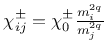
- m1 first eigenvalue of the fabric tensor |
| |
- m2 second eigenvalue of the fabric tensor |
| |
- rho volume fraction of solid phase |
| |
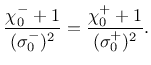
- sig0pos yield stress in tension |
| |
- sig0neg yield stress in compression |
| |
- tau0 yield stress in shear |
| |
- chi0pos interaction coefficient in tension |
| |
- plashardfactor hardening parameter |
| |
- expplashard exponent in hardening law |
| |
- expdam exponent in damage law |
| |
- critdam critical damage |
| |
- expk exponent  in the expression for elastic stiffness in the expression for elastic stiffness |
| |
- expl exponent  in the expression for elastic stiffness in the expression for elastic stiffness |
| |
- expq exponent  in the expression for tensor in the expression for tensor  |
| |
- expp exponent  in the expression for tensor in the expression for tensor |
| Supported modes |
3dMat |

![$\displaystyle =\left[\begin{array}{cccccc}
\frac{1}{E_1} & -\frac{\nu_{12}}{E_1...
...1}{G_{13}} & 0\\
0 & 0 & 0 & 0 & 0 & \frac{1}{G_{12}}
\end{array}\right]^{-1},$](img886.png)
 . Here,
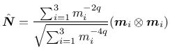
![$\displaystyle =\left[\begin{array}{cccccc}
\frac{1}{\left({\sigma_{1}^{\pm}}\ri...
...}{\tau_{13}} & 0\\
0 & 0 & 0 & 0 & 0 & \frac{1}{\tau_{12}}
\end{array}\right].$](img899.png)
 is the so-called interaction coefficient,