Material for cement hydration - HydratingConcreteMat

Simple hydration models based on chemical affinity are implemented. The models calculate degree of hydration of cement, $\alpha$, which can be scaled to the level of concrete when providing corresponding amount of cement in concrete. Blended cements can be considered as well, either by separating supplementary cementitious materials from pure Portland clinker or by providing parameters for the evolution of hydration degree and potential heat. Released heat from cement paste is obtained from

$$Q(t) = \alpha Q_{pot},$$ (245)

where potential hydration heat, $Q_{pot}$, is expressed in kJ/kg of cement and for pure Portland cement is around 500 kJ/kg.

Evolution of hydration degree under isothemal curing conditions is approximated by several models. Scaling from a reference temperature to arbitrary temperature is based on Arrhenius equation, which coincides with the maturity method approach. The equivalent time, $t_e$, is defined as time under constant reference (isothermal) temperature

$$t_e(T_0) = t(T) k_{rate},$$ (246)

$$k_{rate} = \exp\left[\frac{E_a}{R}\left(\frac{1}{T_0}-\frac{1}{T}\right)\right],$$ (247)

where $t$ is real time, $T$ is the arbitrary constant temperature of hydration, $T_0$ is a reference temperature, $R$ is the universal gas constant (8.314 Jmol$^{-1}$K$^{-1}$) and $E_a$ is the apparent activation energy. Due to varying history of temperature, incremental solution is adopted. Linear and nonlinear nonstationary solvers are supported for all hydrationmodeltype's. Hydration models are evaluated at intrinsic time in each time step. Usually, intrinsic time is in the middle of the time step.

The hydrationmodeltype = 1 is based on exponential approximation of hydration degree [23]. Equivalent time increment is added in each time step. Thus all the thermal history is stored in the equivalent time

$$\alpha(t_e) = \alpha_\infty \exp\left(-\left[\frac{\tau}{t_e} \right]^\beta \right)$$ (248)

where three parameters $\tau$, $\beta$ and $\alpha_\infty$ are needed. Some meaningful parameters are provided in [23], e.g. $\tau=26\cdot3600=93600$ s, $\beta=0.75$ and $\alpha_\infty=0.90$.

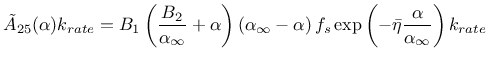
The hydrationmodeltype = 2 is inspired by Cervera et al. [6], who proposed an analytical form of the normalized affinity which was refined in [7]. A slightly modified formulation is proposed here. The affinity model is formulated for a reference temperature 25 $^{\circ}\mathrm{C}$

$$\frac{\mathrm{d}\alpha}{\mathrm{d}t} = \tilde{A}_{25}(\alpha) k_{rate}= B_1 \left( \frac{B_2}{\alpha_\in... ...a \right) f_s \exp\left(-\bar{\eta}\frac{\alpha}{\alpha_\infty}\right) k_{rate}$$ (249)

$$\alpha > DoH_1 \Rightarrow f_s = 1+P_1(\alpha - DoH_1)~\mathrm{else}~f_s = 1$$ (250)

where $B_1, B_2$ are coefficients to be calibrated, $\alpha_\infty$ is the ultimate hydration degree and $\bar{\eta}$ represents microdiffusion of free water through formed hydrates. The function $f_s$ adds additional peak which may occur in slag-rich blended cements with two parameters $DoH_1,P_1$. The solution proceeds incrementally, where $\alpha$ is the unknown. During one macroscopic time step, Eq. (249) needs to be integrated in finer inner steps. This is controlled with two optional variables; maxmodelintegrationtime specifies maximum integration time in the loop while minmodeltimestepintegrations specifies minimum number of integration steps.

Table 58: HydratingConcreteMat - summary of affinity hydration models.

Description	HydratingConcreteMat
Record Format	HydratingConcreteMat num(in) # d(rn) # k(rn) # c(rn) # hydrationmodeltype(in) # Qpot(rn) # masscement(rn) # [activationenergy(rn) #] reinforcementdegree(rn) #] [densitytype(in) #] [conductivitytype(in) #] [capacityType(in) #] [minModelTimeStepIntegrations(in) #] [maxmodelintegrationtime(rn) #] [castingTime(rn) #]
Parameters	- num material model number
	- d material density about 2300 kg/m$^3$
	- k Conductivity about 1.7 W/m/K
	- c Specific heat capacity about 870 J/kg/K
	- hydrationmodeltype 1 is exponential model from Eq. (248), 2 is affinity model from Eq. (249)
	- Qpot Potential heat of hydration, about 500 kJ/kg of cement
	- masscement Cement mass per 1m$^3$ of concrete, about 200-450
	- activationenergy Arrhenius activation energy, 38400. (default)
	- DoHinf degree of hydration at infinite time
	- B1,B2,eta,DoH1,P1 parameters from Eq. (249)-Eq. (250)
	- reinforcementDegree specifies the area fraction of reinforcement. Typical values is 0.015. Steel reinforcement slightly increases concrete conductivity and slightly decreases its capacity. Thermal properties of steel are considered 20 W/m/K and 500 J/kg/K.
	- densityType 0 (default)
	- conductivityType 0 (default), 1 compute as $\lambda = \textrm{k} (1.33-0.33\alpha)$ [21]
	- capacityType 0 (default)
	- minModelTimeStepIntegrations Minimum integrations per time step in affinity model 30 (default)
	- maxmodelintegrationtime Maximum integration time step in affinity model 36000 s (default)
	- castingtime optional casting time of concrete, from which hydration takes place, in s
	- scaling components in the array scale density, conductivity, capacity in this order. nowarnings are checked before scaling.
Supported modes	_2dHeat, _3dHeat

Fig. (15) shows mutual comparison of three hydration models implemented in OOFEM. Parameters for exponential model according to Eq. (248) are $\tau=26\cdot3600=93600$ s, $\beta=0.75$, $\alpha_\infty=0.90$. Parameters for affinity model according to Eq. (249) are $B_1=3.519e-4$ s$^{-1}$, $B_2=8.0e-7$, $\eta=7.4$, $\alpha_\infty=0.85$.

Figure 15: Performance of implemented hydration models: exponential model from Eq. (248), affinity model from Eq. (249), CEMHYD3D model from Subsection 2.5.