Examples

Beam structure

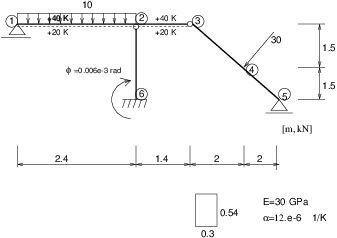
This example for a simple beam structure gives basic overview of the input file (found under tests/sm/beam2d_1.in). Structure geometry and its constitutive and geometrical properties are shown in Fig. (ex01). The linear static analysis is required, the influence of shear is neglected.

Example 1 - beam2d_1.in

beam2d_1.out
Simple Beam Structure - linear analysis
#only momentum influence to the displacements is taken into account
#beamShearCoeff is artificially enlarged.
StaticStructural nsteps 3 nmodules 0
domain 2dBeam
OutputManager tstep_all dofman_all element_all
ndofman 6 nelem 5 ncrosssect 1 nmat 1 nbc 6 nic 0 nltf 3 nset 7
node 1 coords 3 0.  0.  0.
node 2 coords 3 2.4 0.  0.
node 3 coords 3 3.8 0.  0.
node 4 coords 3 5.8 0.  1.5
node 5 coords 3 7.8 0.  3.0
node 6 coords 3 2.4 0.  3.0
Beam2d 1 nodes 2 1 2
Beam2d 2 nodes 2 2 3 DofsToCondense 1 6
Beam2d 3 nodes 2 3 4 DofsToCondense 1 3
Beam2d 4 nodes 2 4 5
Beam2d 5 nodes 2 6 2 DofsToCondense 1 6
SimpleCS 1 area 1.e8 Iy 0.0039366 beamShearCoeff 1.e18 thick 0.54 material 1 set 1
IsoLE 1 d 1. E 30.e6 n 0.2 tAlpha 1.2e-5
BoundaryCondition 1 loadTimeFunction 1 dofs 1 3 values 1 0.0 set 4
BoundaryCondition 2 loadTimeFunction 1 dofs 1 5 values 1 0.0 set 5
BoundaryCondition 3 loadTimeFunction 2 dofs 3 1 3 5 values 3 0.0 0.0 -0.006e-3 set 6
ConstantEdgeLoad 4 loadTimeFunction 1 Components 3 0.0 10.0 0.0 loadType 3 set 3
NodalLoad 5 loadTimeFunction 1 dofs 3 1 3 5 Components 3 -18.0 24.0 0.0 set 2
StructTemperatureLoad 6 loadTimeFunction 3 Components 2 30.0 -20.0 set 7
PeakFunction 1 t 1.0 f(t) 1.
PeakFunction 2 t 2.0 f(t) 1.
PeakFunction 3 t 3.0 f(t) 1.
Set 1 elementranges {(1 5)}
Set 2 nodes 1 4
Set 3 elementedges 2 1 1
Set 4 nodes 2 1 5
Set 5 nodes 1 3
Set 6 nodes 1 6
Set 7 elements 2 1 2

Plane stress example

Example 2

patch100.out
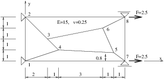
Patch test of PlaneStress2d elements -> pure compression
LinearStatic nsteps 1
domain 2dPlaneStress
OutputManager tstep_all dofman_all element_all
ndofman 8 nelem 5 ncrosssect 1 nmat 1 nbc 3 nic 0 nltf 1 nset 3
node 1 coords 3  0.0   0.0   0.0
node 2 coords 3  0.0   4.0   0.0
node 3 coords 3  2.0   2.0   0.0
node 4 coords 3  3.0   1.0   0.0
node 5 coords 3  8.0   0.8   0.0
node 6 coords 3  7.0   3.0   0.0
node 7 coords 3  9.0   0.0   0.0
node 8 coords 3  9.0   4.0   0.0
PlaneStress2d 1 nodes 4 1 4 3 2  NIP 1
PlaneStress2d 2 nodes 4 1 7 5 4  NIP 1
PlaneStress2d 3 nodes 4 4 5 6 3  NIP 1
PlaneStress2d 4 nodes 4 3 6 8 2  NIP 1
PlaneStress2d 5 nodes 4 5 7 8 6  NIP 1
Set 1 elementranges {(1 5)}
Set 2 nodes 2 1 2
Set 3 nodes 2 7 8
SimpleCS 1 thick 1.0 width 1.0 material 1 set 1
IsoLE 1 d 0. E 15.0 n 0.25 talpha 1.0
BoundaryCondition 1 loadTimeFunction 1 dofs 2 1 2 values 1 0.0 set 2
BoundaryCondition 2 loadTimeFunction 1 dofs 1 2 values 1 0.0 set 3
NodalLoad 3 loadTimeFunction 1 dofs 2 1 2 components 2 2.5 0.0 set 3
ConstantFunction 1 f(t) 1.0

Examples - parallel mode

Node-cut example

The example shows explicit direct integration analysis of simple structure with two DOFs. The geometry and partitioning is sketched in fig.(nodecut-ex01).

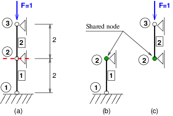
Node-cut partitioning example: (a) whole geometry, (b) partition 0, (c) partition 1.

#
# partition 0
#
partest.out.0
Parallel test of explicit oofem computation
#
NlDEIDynamic nsteps 3 dumpcoef 0.0 deltaT 1.0
domain 2dTruss
#
OutputManager tstep_all dofman_all element_all
ndofman 2 nelem 1 ncrosssect 1 nmat 1 nbc 3 nic 0 nltf 1 nset 4
#
Node 1 coords 3 0. 0. 0.
Node 2 coords 3 0. 0. 2. Shared partitions 1 1
Truss2d 1 nodes 2 1 2
Set 1 elements 1 1
Set 2 nodes 2 1 2
Set 3 nodes 1 1
Set 4 nodes 0
SimpleCS 1 thick 0.1 width 10.0 material 1 set 1
IsoLE 1 tAlpha 0.000012 d 10.0 E 1.0 n 0.2
BoundaryCondition 1 loadTimeFunction 1 dofs 1 1 values 1 0.0 set 2
BoundaryCondition 2 loadTimeFunction 1 dofs 1 3 values 1 0.0 set 3
NodalLoad 3 loadTimeFunction 1 dofs 2 1 3 components 2 0. 1.0 set 4
ConstantFunction 1 f(t) 1.0

#
# partition 1
#
partest.out.1
Parallel test of explicit oofem computation
#
NlDEIDynamic nsteps 3 dumpcoef 0.0 deltaT 1.0
domain 2dTruss
#
OutputManager tstep_all dofman_all element_all
ndofman 2 nelem 1 ncrosssect 1 nmat 1 nbc 3 nic 0 nltf 1 nset 4
#
Node 2 coords 3 0. 0. 2. Shared partitions 1 0
Node 3 coords 3 0. 0. 4.
Truss2d 2 nodes 2 2 3
Set 1 elements 1 2
Set 2 nodes 2 2 3
Set 3 nodes 0
Set 4 nodes 1 3
SimpleCS 1 thick 0.1 width 10.0 material 1 set 1
IsoLE 1 tAlpha 0.000012 d 10.0 E 1.0 n 0.2
BoundaryCondition 1 loadTimeFunction 1 dofs 1 1 values 1 0.0 set 2
BoundaryCondition 2 loadTimeFunction 1 dofs 1 3 values 1 0.0 set 3
NodalLoad 3 loadTimeFunction 1 dofs 2 1 3 components 2 0. 1.0 set 4
ConstantFunction 1 f(t) 1.0

Element-cut example

The example shows explicit direct integration analysis of simple structure with two DOFs. The geometry and partitioning is sketched in fig. (nodecut-ex01).

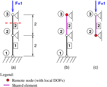
Element-cut partitioning example: (a) whole geometry, (b) partition 0, (c) partition 1.

#
# partition 0
#
partest2.out.0
Parallel test of explicit oofem computation
#
NlDEIDynamic nsteps 5 dumpcoef 0.0 deltaT 1.0
domain 2dTruss
#
OutputManager tstep_all dofman_all element_all
ndofman 3 nelem 2 ncrosssect 1 nmat 1 nbc 3 nic 0 nltf 1 nset 4
#
Node 1 coords 3 0. 0. 0.
Node 2 coords 3 0. 0. 2.
Node 3 coords 3 0. 0. 4. Remote partitions 1 1
Truss2d 1 nodes 2 1 2
Truss2d 2 nodes 2 2 3
Set 1 elements 2 1 2
Set 2 nodes 3 1 2 3
Set 3 nodes 1 1
Set 4 nodes 1 3
SimpleCS 1 thick 0.1 width 10.0 material 1 set 1
IsoLE 1 tAlpha 0.000012 d 10.0 E 1.0 n 0.2
BoundaryCondition 1 loadTimeFunction 1 dofs 1 1 values 1 0.0 set 2
BoundaryCondition 2 loadTimeFunction 1 dofs 1 3 values 1 0.0 set 3
NodalLoad 3 loadTimeFunction 1 dofs 2 1 3 components 2 0. 1.0 set 4
ConstantFunction 1 f(t) 1.0


#
# partition 1
#
partest2.out.1
Parallel test of explicit oofem computation
#
NlDEIDynamic nsteps 5 dumpcoef 0.0 deltaT 1.0
domain 2dTruss
#
OutputManager tstep_all dofman_all element_all
ndofman 2 nelem 1 ncrosssect 1 nmat 1 nbc 3 nic 0 nltf 1 nset 4
#
Node 2 coords 3 0. 0. 2 Remote partitions 1 0
Node 3 coords 3 0. 0. 4
Truss2d 2 nodes 2 2 3
Set 1 elements 1 2
Set 2 nodes 2 2 3
Set 3 nodes 0
Set 4 nodes 1 3
SimpleCS 1 thick 0.1 width 10.0 material 1 set 1
IsoLE 1 tAlpha 0.000012 d 10.0 E 1.0 n 0.2
BoundaryCondition 1 loadTimeFunction 1 dofs 1 1 values 1 0.0 set 2
BoundaryCondition 2 loadTimeFunction 1 dofs 1 3 values 1 0.0 set 3
NodalLoad 3 loadTimeFunction 1 dofs 2 1 3 components 2 0. 1.0 set 4
ConstantFunction 1 f(t) 1.0

Figures

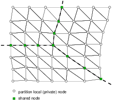
Node-cut partitioning.

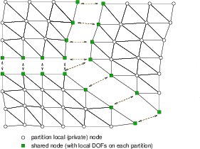
Node-cut partitioning - local constitutive mode.

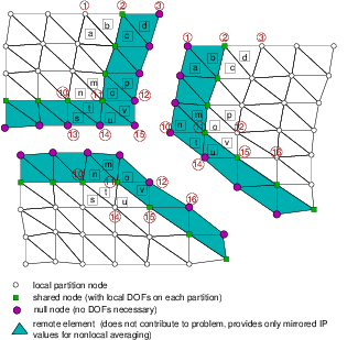
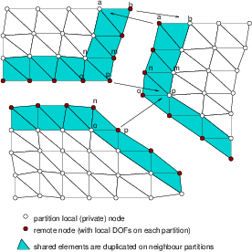
Node-cut partitioning - nonlocal constitutive mode.

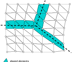
Element-cut partitioning.

Element-cut partitioning, local constitutive mode.

[1]

Hovewer, the problem does not support the changes of static system. But it is possible to apply direct displacement control without requiring BC applied (see nrsolver documentation). Therefore it is possible to combine direct displacement control with direct load control or indirect control.