Next: Heat flux from radiation Up: Solution procedures Previous: Non-stationary linear transport model Contents
Time discretization is the same as in but the assumption in Eq. (2.15) is not true anymore. Let us assume that Eq. (2.16) should be satisfied at time
![]() . By substituting of into Eq. (2.16) leads to the following equation
. By substituting of into Eq. (2.16) leads to the following equation
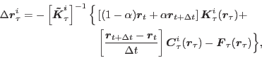
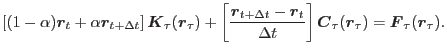
Eq. (2.17) is non-linear and the Newton method is used to obtain the solution. First, the Eq. (2.17) is
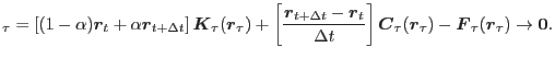
transformed into a residual form with the residuum vector
![]()
![]() , which should converge to the zero vector
, which should converge to the zero vector
A new residual vector at the next iteration,
![]()
![]() , can determined from the previous residual vector,
, can determined from the previous residual vector,
![]()
![]() , and its derivative simply by linearization. Since the aim is getting an increment of solution vector,
, and its derivative simply by linearization. Since the aim is getting an increment of solution vector,
![]()
![]()
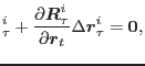
![]() , the new residual vector
, the new residual vector
![]()
![]() is set to zero
is set to zero
There are two options how to initialize the solution vector at time
![]() . While the first case applies linearization with a known derivative, the second case simply starts from the previous solution vector. The second method in Eq. (2.26) is implemented in OOFEM.
. While the first case applies linearization with a known derivative, the second case simply starts from the previous solution vector. The second method in Eq. (2.26) is implemented in OOFEM.
Note that the matrices
![]()
![]()
![]()
![]()
![]()
![]()
![]()
![]() and the vector
and the vector
![]()
![]()
![]()
![]() depend on the solution vector
depend on the solution vector
![]()
![]() . For this reason, the matrices are updated in each iteration step (Newton method) or only after several steps (modified Newton method). The residuum
. For this reason, the matrices are updated in each iteration step (Newton method) or only after several steps (modified Newton method). The residuum
![]()
![]() and the vector
and the vector
![]()
![]()
![]()
![]() are updated in each iteration, using the most recent capacity and conductivity matrices.
are updated in each iteration, using the most recent capacity and conductivity matrices.

![$\displaystyle - \left[\frac{\partial{\mbox{\boldmath$R$}_{\tau}^i}}{\partial\mbox{\boldmath$r$}_t}\right]^{-1} \mbox{\boldmath$R$}_{\tau}^i.$](img279.png)
![$\displaystyle - \left[\mbox{\boldmath$\tilde K$}_\tau^i\right]^{-1} \mbox{\boldmath$R$}_{\tau}^i,$](img283.png)