Next: Nonlocal formulation Up: Anisotropic damage model - Previous: Anisotropic damage model -
The concept of isotropic damage is appropriate for materials weakened by voids, but if the physical source of damage is the initiation and propagation of microcracks, isotropic stiffness degradation can be considered only as a first rough approximation. More refined damage models take into account the highly oriented nature of cracking, which is reflected by the anisotropic character of the damaged stiffness or compliance matrices.
A number of anisotropic damage formulations have been proposed in the literature. Here we use a model outlined by Jirásek [16], which is based on the principle of energy equivalence and on the construction of the inverse integrity tensor by integration of a scalar over all spatial directions. Since the model uses certain concepts from the microplane theory, it is called the microplane-based damage model (MDM).
The general structure of the MDM
model is schematically shown in Fig. 7
and the basic equations are summarized in Tab. 26.
Here,
![]() and
and
![]() are the (nominal) second-order
strain and stress tensors
with components
are the (nominal) second-order
strain and stress tensors
with components
![]()
![]() and
and
![]() ;
;
![]() and
and
![]() are first-order strain and stress tensors with components
are first-order strain and stress tensors with components ![]() and
and ![]() , which characterize the strain and stress on “microplanes”
of different orientations given by a unit vector
, which characterize the strain and stress on “microplanes”
of different orientations given by a unit vector
![]() with components
with components ![]() ;
;
![]() is a dimensionless compliance parameter
that is a scalar but can have different values for different
directions
is a dimensionless compliance parameter
that is a scalar but can have different values for different
directions
![]() ;
the symbol
;
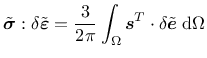
the symbol ![]() denotes a virtual quantity; and a sumperimposed
tilde denotes an effective quantity, which is supposed to characterize the
state of the intact material between defects such as microcracks or voids.
denotes a virtual quantity; and a sumperimposed
tilde denotes an effective quantity, which is supposed to characterize the
state of the intact material between defects such as microcracks or voids.
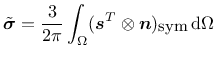
Combining the basic equations, it is possible to show that the components of the damaged material compliance tensor are given by
The scalar variable ![]() characterizes the relative compliance
in the direction given by the vector
characterizes the relative compliance
in the direction given by the vector
![]() .
If
.
If ![]() is the same in all directions,
the inverse integrity tensor evaluated from (82)
is equal to the unit second-order tensor (Kronecker delta) multiplied
by
is the same in all directions,
the inverse integrity tensor evaluated from (82)
is equal to the unit second-order tensor (Kronecker delta) multiplied
by ![]() , the damage effect tensor evaluated from (81)
is equal to the symmetric fourth-order unit tensor multiplied
by
, the damage effect tensor evaluated from (81)
is equal to the symmetric fourth-order unit tensor multiplied
by ![]() ,
and the damaged
material compliance tensor evaluated from (80) is the
elastic compliance tensor multiplied by
,
and the damaged
material compliance tensor evaluated from (80) is the
elastic compliance tensor multiplied by ![]() . The factor multiplying
the elastic compliance tensor in the
isotropic damage model is
. The factor multiplying
the elastic compliance tensor in the
isotropic damage model is
![]() , and so
, and so ![]() corresponds
to
corresponds
to
![]() . In the initial undamaged state,
. In the initial undamaged state,
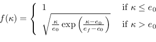
![]() in all directions. The evolution of
in all directions. The evolution of ![]() is governed by the history of the projected strain components.
In the simplest case,
is governed by the history of the projected strain components.
In the simplest case, ![]() is driven by the normal strain
is driven by the normal strain
![]()
![]()
![]() . Analogy with the isotropic damage model
leads to the damage law
. Analogy with the isotropic damage model
leads to the damage law
| (83) |
| (84) |
If the MDM model is used in its basic form described above,
the compressive strength turns out to depend on the Poisson ratio and,
in applications to concrete, its value is too low compared to the
tensile strength. The model is designed primarily for tensile-dominated
failure, so the low compressive strength
is not considered as a major drawback. Still, it
is desirable to introduce a modification that would prevent spurious
compressive failure in problems where moderate compressive stresses
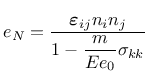
appear. The desired effect is achieved by redefining the projected
strain ![]() as
as
Borek Patzak


![\includegraphics[width=0.8\textwidth]{dm_comp.eps}](img373.png)
 d
d