Damage-plastic model for concrete - ConcreteDPM
This model, developed by Grassl and Jirásek for failure of concrete
under general triaxial stress, is described in detail in [8].
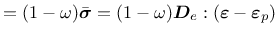
It belongs to the class of damage-plastic models with yield condition formulated
in terms of the effective stress
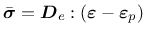 .
The stress-strain law is postulated in the form
.
The stress-strain law is postulated in the form
  |
(141) |
where

 is the elastic stiffness tensor
and
is the elastic stiffness tensor
and  is a scalar damage parameter.
The plastic part of the model consists of a three-invariant yield condition, nonassociated flow rule and pressure-dependent hardening law.
For simplicity, damage is assumed to be isotropic.
In contrast to pure damage models with damage driven by the total strain, here the damage is linked to the evolution of plastic strain.
is a scalar damage parameter.
The plastic part of the model consists of a three-invariant yield condition, nonassociated flow rule and pressure-dependent hardening law.
For simplicity, damage is assumed to be isotropic.
In contrast to pure damage models with damage driven by the total strain, here the damage is linked to the evolution of plastic strain.
The yield surface is described in terms of the cylindrical coordinates in the principal effective stress space (Haigh-Westergaard coordinates), which are the volumetric effective stress
 , the norm of the deviatoric effective stress
 ,
and the Lode angle
,
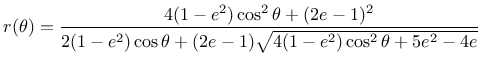
and the Lode angle  defined by the relation
 |
(142) |
where  and
and  are the second and third deviatoric invariants.
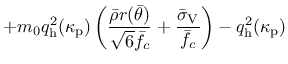
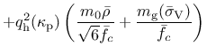
The yield function
are the second and third deviatoric invariants.
The yield function
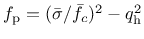
depends on the effective stress (which enters in the form of cylindrical coordinates) and on the hardening variable
 (which enters through a dimensionless variable
  ). Parameter
  is the uniaxial compressive strength.
Note that, under uniaxial compression characterized by axial stress
is the uniaxial compressive strength.
Note that, under uniaxial compression characterized by axial stress
 , we have
 ,
,
 and
and
 . The yield function
then reduces to
. The yield function
then reduces to
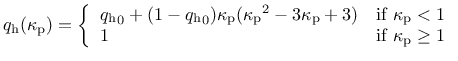
 . This means that
function
. This means that
function
 describes the evolution of the uniaxial compressive
yield stress normalized by its maximum value, .
describes the evolution of the uniaxial compressive
yield stress normalized by its maximum value, .
The evolution of the yield surface during hardening is presented in Fig. 8.
The parabolic shape of the meridians (Fig. 8a) is controlled by the hardening variable and the friction parameter  .
The initial yield surface is closed, which allows modeling of compaction under highly confined compression. The initial and intermediate
yield surfaces have two vertices on the hydrostatic axis but the ultimate yield surface has only one vertex
on the tensile part of the hydrostatic axis and opens up along the compressive
part of the hydrostatic axis.
The deviatoric sections evolve as shown in Fig. 8b,
and their final shape at full hardening
is a rounded triangle at low confinement and almost circular
at high confinement.
The shape of the deviatoric section is controlled by the Willam-Warnke
function
.
The initial yield surface is closed, which allows modeling of compaction under highly confined compression. The initial and intermediate
yield surfaces have two vertices on the hydrostatic axis but the ultimate yield surface has only one vertex
on the tensile part of the hydrostatic axis and opens up along the compressive
part of the hydrostatic axis.
The deviatoric sections evolve as shown in Fig. 8b,
and their final shape at full hardening
is a rounded triangle at low confinement and almost circular
at high confinement.
The shape of the deviatoric section is controlled by the Willam-Warnke
function
 |
(144) |
The eccentricity parameter  that appears in this function, as well as the friction parameter , are calibrated from the values of uniaxial and equibiaxial compressive strengths and uniaxial tensile strength.
Figure:
Evolution of the yield surface during hardening:
a) meridional section, b) deviatoric section for a constant volumetric effective stress of

 |
The maximum size of the elastic domain is attained when the variable is equal to one (which is its maximum value, as follows from the hardening law, to be specified in (149)). The yield surface is then described by the equation
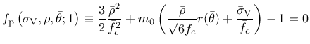 |
(145) |
The flow rule
 |
(146) |
is non-associated, which means that the yield function  and the plastic potential
do not coincide and, therefore, the direction of the plastic flow
 is not normal to the yield surface.
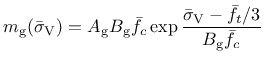
The ratio of the volumetric and the deviatoric parts of the flow direction is controled by function
is not normal to the yield surface.
The ratio of the volumetric and the deviatoric parts of the flow direction is controled by function  , which depends on the volumetric stress and is defined as
 |
(148) |
where  and
and  are model parameters that are determined from certain assumptions on the plastic flow in uniaxial tension and compression.
The dimensionless variable that appears in the yield function (143) is a function of the hardening variable
. It controls the size and shape of the yield surface and, thereby, of the elastic domain.
The hardening law is given by
 |
(149) |
The initial inclination of the hardening curve (at
 ) is positive and finite, and the inclination at peak (i.e., at
 ) is zero.
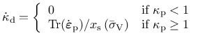
The evolution law for the hardening variable,2
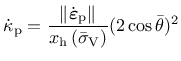 |
(150) |
sets the rate of the hardening variable equal to the norm of the plastic strain rate
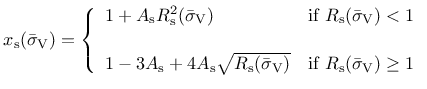
scaled by a hardening ductility measure
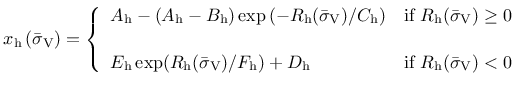 |
(151) |
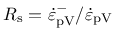
The dependence of the scaling factor
 on the volumetric effective stress
 is constructed such that
the model response is more ductile under compression.
The variable
is constructed such that
the model response is more ductile under compression.
The variable
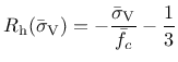 |
(152) |
is a linear function of the volumetric effective stress.
Model parameters
 and
and  are calibrated from the values of strain at peak stress under uniaxial tension, uniaxial compression and triaxial compression, whereas the parameters
are determined from the conditions of a smooth transition between the two parts of equation (151) at
 .
.
For the present model, the evolution of damage starts after full saturation of plastic hardening, i.e., at
. This greatly facilitates calibration of model parameters, because the strength envelope is fully controled by the plastic part of the model and damage affects only the softening behavior.
In contrast to pure damage models,
damage is assumed to be driven by the plastic strain, more
specifically by its volumetric part, which is closely related
to cracking. To slow down the evolution of damage under compressive stress states,
the damage-driving variable
 is not set equal to the volumetric
plastic strain, but it is defined incrementally by the rate equation
is not set equal to the volumetric
plastic strain, but it is defined incrementally by the rate equation
 |
(155) |
where
 |
(156) |
is a softening ductility measure.
Parameter  is determined from the softening response in uniaxial compression. The dimensionless variable
 is defined as the ratio between the “negative” volumetric plastic strain rate
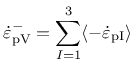 |
(157) |
and the total volumetric plastic strain rate
 .
This ratio depends only on the flow direction
, and thus
.
This ratio depends only on the flow direction
, and thus
 can be shown to be a unique function of the volumetric effective stress. In (157),
 are the principal components of the rate of plastic strains and
 denotes the McAuley brackets (positive-part operator).
For uniaxial tension, for instance, all three principal plastic strain rates are nonnegative, and so
denotes the McAuley brackets (positive-part operator).
For uniaxial tension, for instance, all three principal plastic strain rates are nonnegative, and so
 ,
,
 and
and
 . This means that under uniaxial tensile loading we have
 . On the other hand, under compressive stress states the negative principal plastic strain rates lead to a ductility measure
  greater than one and the evolution of damage is slowed down. It should be emphasized that the flow rule for this specific model is constructed such that the volumetric part of plastic strain rate at the ultimate yield surface cannot be negative.
Table 40:
Damage-plastic model for concrete - summary.
| Description |
Damage-plastic model for concrete |
| Record Format |
ConcreteDPM d(rn) #
E(rn) # n(rn) # tAlpha(rn) #
ft(rn) # fc(rn) # wf(rn) # Gf(rn) # ecc(rn) #
kinit(rn) # Ahard(rn) # Bhard(rn) # Chard(rn) # Dhard(rn) # Asoft(rn) # helem(rn) # href(rn) # dilation(rn) # yieldtol(rn) # newtoniter(in) # |
| Parameters |
- d material density |
| |
- E Young modulus |
| |
- n Poisson ratio |
| |
- tAlpha thermal dilatation coefficient |
| |
- ft uniaxial tensile strength  |
| |
- fc uniaxial compressive strength |
| |
- wf parameter  that controls the slope of the softening branch (serves for the evaluation of that controls the slope of the softening branch (serves for the evaluation of
  to be used in (158)) to be used in (158)) |
| |
- Gf fracture energy, can be specified instead of wf, it is converted to
 |
| |
- ecc eccentricity parameter from (144), optional, default value 0.525 |
| |
- kinit parameter
 from (149), optional, default value 0.1 from (149), optional, default value 0.1 |
| |
- Ahard parameter  from (151), optional, default value 0.08 from (151), optional, default value 0.08 |
| |
- Bhard parameter  from (151), optional, default value 0.003 from (151), optional, default value 0.003 |
| |
- Chard parameter  from (151), optional, default value 2 from (151), optional, default value 2 |
| |
- Dhard parameter from (151), optional, default value  |
| |
- Asoft parameter from (156), optional, default value 15 |
| |
- helem element size  , optional (if not specified, the actual element size is used) , optional (if not specified, the actual element size is used) |
| |
- href reference element size  , optional (if not specified, the standard adjustment of the damage law is used) , optional (if not specified, the standard adjustment of the damage law is used) |
| |
- dilation dilation factor (ratio between lateral and axial plastic strain rates in the softening regime under uniaxial compression), optional, default value -0.85 |
| |
- yieldtol tolerance for the implicit stress return algorithm, optional, default value  |
| |
- newtoniter maximum number of iterations in the implicit stress return algorithm, optional, default value 100 |
| Supported modes |
3dMat |
|
The relation between the damage variable and the internal variable
(maximum level of equivalent strain) is assumed to have the exponential form
 |
(158) |
where
 is a parameter that controls the slope of the softening curve. In fact, equation (158) is used by the nonlocal version
of the damage-plastic model, with
replaced by its weighted
spatial average (not yet available in the public version of OOFEM).
For the local model, it is necessary to adjust softening according
to the element size, otherwise the results would suffer by pathological
mesh sensitivity. It is assumed that localization takes place at the
peak of the stress-strain diagram, i.e., at the onset of damage.
After that, the strain is decomposed into the distributed
part, which corresponds to unloading from peak, and the localized part,
which is added if the material is softening.
The localized part of strain
is transformed into an equivalent crack opening,
is a parameter that controls the slope of the softening curve. In fact, equation (158) is used by the nonlocal version
of the damage-plastic model, with
replaced by its weighted
spatial average (not yet available in the public version of OOFEM).
For the local model, it is necessary to adjust softening according
to the element size, otherwise the results would suffer by pathological
mesh sensitivity. It is assumed that localization takes place at the
peak of the stress-strain diagram, i.e., at the onset of damage.
After that, the strain is decomposed into the distributed
part, which corresponds to unloading from peak, and the localized part,
which is added if the material is softening.
The localized part of strain
is transformed into an equivalent crack opening,  , which is
under uniaxial tension linked
to the stress by the exponential law
, which is
under uniaxial tension linked
to the stress by the exponential law
 |
(159) |
Here, is the uniaxial tensile strength and is the characteristic
crack opening, playing a similar role to
.
Under uniaxial tension, the localized strain can be expressed as the sum
of the post-peak plastic strain (equal to variable
)
and the unloaded part of elastic strain (equal to
 ).
Denoting the effective element size as , we can write
).
Denoting the effective element size as , we can write
 |
(160) |
and substituting this into (159), we obtain a nonlinear
equation
 |
(161) |
from which the damage variable corresponding to the given internal
variable
can be computed by Newton iteration.
The effective element size is obtained by projecting the element onto
the direction of the maximum principal strain at the onset of cracking,
and afterwards it is held fixed. The evaluation of from
is no longer explicit, but the resulting load-displacement curve
of a bar under uniaxial tension is totally independent of the mesh size.
A simpler approach would be to use (158) with
 , but then the scaling would not be perfect and
the shape of the load-displacement curve (and also the dissipated energy)
would slightly depend on the mesh size. With the present approach,
the energy per unit sectional area dissipated under uniaxial tension
is exactly
, but then the scaling would not be perfect and
the shape of the load-displacement curve (and also the dissipated energy)
would slightly depend on the mesh size. With the present approach,
the energy per unit sectional area dissipated under uniaxial tension
is exactly
 . The input parameter controling the damage law
can be either the characteristic crack opening ,
or the fracture energy
. The input parameter controling the damage law
can be either the characteristic crack opening ,
or the fracture energy  . If both are specified, is used and
is ignored. If only is specified, is set to
. If both are specified, is used and
is ignored. If only is specified, is set to  .
.
The onset of damage corresponds to the peak of the stress-strain diagram
under proportional loading, when the ratios of the stress components are fixed.
This is the case e.g. for uniaxial tension, uniaxial compression, or shear
under free expansion of the material (with zero normal stresses). However,
for shear under confinement the shear stress can rise even after the onset
of damage, due to increasing hydrostatic pressure, which increases the
mobilized friction. It has been observed that the standard approach leads
to strong sensitivity of the peak shear stress to the element size.
To reduce this pathological effect, a modified approach has been implemented.
The second-order work (product of stress increment and strain increment)
is checked after each step and the element-size dependent adjustment
of the damage law is applied only after the second-order work becomes negative.
Up to this stage, the damage law corresponds to a fixed reference element
size, which is independent of the actual size of the element.
This size is set by the optional parameter href.
If this parameter is not specified, the standard approach is used.
For testing purposes, one can also specify the actual element size,
helem, as a “material property”. If this parameter is not
specified, the element size is computed for each element separately
and represents its actual size.
The damage-plastic model contains 15 parameters, but only 6 of them need to be actually calibrated for different concrete types, namely Young's modulus  , Poisson's ratio
  , tensile strength
  , compressive strength
  , parameter (or fracture energy ), and parameter in the ductility measure (156) of the damage model. The remaining parameters can be set to their default values specified in [8].
The model parameters are summarized
in Tab. 40. Note that it is possible to specify the “size” of finite element, , which (if specified) replaces
the actual element size in (161). The usual approach is to consider as the actual element size (evaluated automatically by OOFEM),
in which case the optional
parameter is missing (or is set to 0., which has the same effect in the code). However, for various studies of mesh sensitivity
it is useful to have the option of specifying as an input “material” value.
If the element is too large, it may become too brittle and local snap-back
occurs in the stress-strain diagram, which is not acceptable.
In such a case, an error message is issued and the program execution
is terminated. The maximum admissible element size
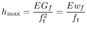 |
(162) |
happens to be equal to Hillerborg's characteristic material length.
For typical concretes it is in the order of a few hundred mm.
If the condition
 is violated, the mesh needs to be refined.
Note that the effective element size is obtained by projecting the element.
For instance, if the element is a cube of edge length 100 mm, its effective
size in the direction of the body diagonal can be 173 mm.
is violated, the mesh needs to be refined.
Note that the effective element size is obtained by projecting the element.
For instance, if the element is a cube of edge length 100 mm, its effective
size in the direction of the body diagonal can be 173 mm.
Borek Patzak
2019-03-19
![$\displaystyle \left(\left[1-q_{\rm {h}}(\kappa_{\rm p})\right]\left( \frac{\bar...
...{f}_c} \right)^2 + \sqrt{\frac{3}{2}} \frac {\bar{\rho}}{\bar{f}_c} \right)^2 +$](img653.png)