This model is an extension of the ConcreteDPM presented in 1.6.9.
CDPM2 has been developed by Grassl, Xenos, Nyström, Rempling and Gylltoft for modelling the failure of concrete for both static and dynamic loading. It is is described in detail in [9].
The main differences between CDPM2 and ConcreteDPM are that in CDPM2 the plasticity part exhibits hardening once damage is active. Furthermore, two independent damage parameters describing tensile and compressive damage are introduced.
The parameters of CDPM2 are summarised in Tab. 41
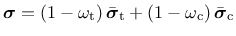
The stress for the anisotropic damage plasticity model (ISOFLAG=0) is defined as
 |
(163) |
where
 and
and
 are the positive and negative parts of the effective stress tensor
 , respectively, and
 and
and
 are two scalar damage variables, ranging from 0 (undamaged) to 1 (fully damaged).
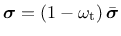
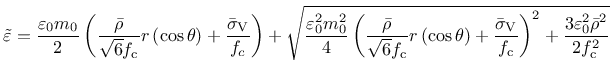
The stress for the isotropic damage plasticity model (ISOFLAG=1) is defined as
 |
(164) |
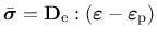
The effective stress
is defined according to the damage mechanics convention as
 |
(165) |
Plasticity:
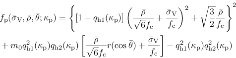
The yield surface is described by the Haigh-Westergaard coordinates: the volumetric effective stress
 , the norm of the deviatoric effective stress
  and the Lode angle
  . The yield surface is
 |
(166) |
It depends also on the hardening variable
 (which enters through the dimensionless variables
 and
and
 ). Parameter
  is the uniaxial compressive strength. For
 , the yield function is identical to the one of CDPM.
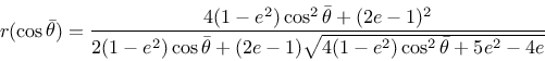
The shape of the deviatoric section is controlled by the Willam-Warnke function
, the yield function is identical to the one of CDPM.
The shape of the deviatoric section is controlled by the Willam-Warnke function
 |
(167) |
Here,  is the eccentricity parameter.
The friction parameter
is the eccentricity parameter.
The friction parameter  is given by
 |
(168) |
where  is the tensile strength.
The flow rule (26) is split into a volumetric and a deviatoric part, i.e., the gradient of the plastic potential is decomposed as
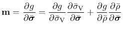 |
(169) |
Taking into account that
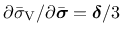 and
and
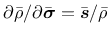 , restricting attention to the post-peak regime (in which
 ) and differentiating the plastic potential (147), we rewrite equation (169) as
  |
(170) |
The flow rule is non-associative which means that the direction of the plastic flow is not normal to the yield surface. This is important for concrete since an associative flow rule would give an overestimated maximum stress for passive confinement.
The dimensionless variables
and
that appear in (143), (147) and (148) are functions of the hardening variable
. They control the evolution of the size and shape of the yield surface and plastic potential.
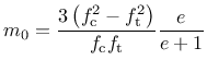
The first hardening law
is
 |
(171) |
The second hardening law
is given by
 |
(172) |
The evolution law for the hardening variable,
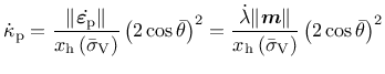 |
(173) |
sets the rate of the hardening variable equal to the norm of the plastic strain rate scaled by a hardening ductility measure, which is identical to the one used for the CDPM.
Damage:
Damage is initiated when the maximum equivalent strain in the history of the material reaches the threshold
 .
This expression is determined from the yield surface (
.
This expression is determined from the yield surface (
 ) by setting
 and
and
 .
From this quadratic equation for
.
From this quadratic equation for
 , the equivalent strain is determined as
 |
(174) |
Tensile damage is described by a stress-inelastic displacement law. For linear and exponential damage type the stress value and the displacement value  must be defined. For the bi-linear type two additional parameters
 and
and
 are required.
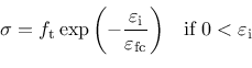
For the compressive damage variable, an evolution based on an exponential stress-inelastic strain law is used. The stress versus inelastic strain in the softening regime in compression is
 |
(175) |
where
 is an inelastic strain threshold which controls the initial inclination of the softening curve. The use of different damage evolution for tension and compression is one important improvement over CDPM.
The history variables
 ,
,
 ,
,
 and
and
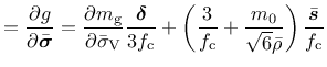
 depend on a ductility measure
  , which takes into account the influence of multiaxial stress states on the damage evolution.
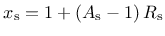
This ductility measure is given by
, which takes into account the influence of multiaxial stress states on the damage evolution.
This ductility measure is given by
 |
(176) |
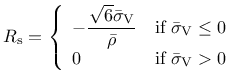
where  is
is
 |
(177) |
and  is a model parameter.
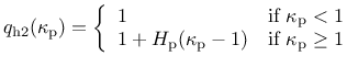
Strain rate:
Concrete is strongly rate dependent. If the loading rate is increased, the tensile and compressive strength increase and are more prominent in tension then in compression. The dependency is taken into account by an additional variable
 . The rate dependency is included by scaling both the equivalent strain rate and the inelastic strain. The rate parameter is defined by
 |
(178) |
where  is the continuous compression measure (= 1 means only compression, = 0 means only tension).
The functions
 and
and
 depend on the input parameter
 . A recommended value for
is 10 MPa.
. A recommended value for
is 10 MPa.
Table 41:
CDPM2 - summary.
| Description |
CDPM2 |
| Record Format |
con2dpm d(rn) # E(rn) # n(rn) # tAlpha(rn) # ft(rn) # fc(rn) # wf(rn) # [stype(in) #] [ft1(rn) #] [wf1(rn) #] [efc(rn) #] [ecc(rn) #] [kinit(rn) #] [Ahard(rn) #] [Bhard(rn) #] [Chard(rn) #] [Dhard(rn) #] [Asoft(rn) #] [helem(rn) #] [dilation(rn) #] [hp(rn) #] [isoflag(in) #] [rateflag(in) #] fcZero(in) # [yieldtol(rn) #] [newtoniter(in) #] |
| Parameters |
- d material density |
| |
- E Young modulus |
| |
- n Poisson ratio |
| |
- tAlpha thermal dilatation coefficient |
| |
- ft uniaxial tensile strength |
| |
- fc uniaxial compressive strength |
| |
- wf parameter that controls the slope of the softening branch to be used |
| |
- stype allows to choose different types of softening laws, default value 1:
| 0 - | linear softening |
| 1 - | bilinear softening |
| 2 - | exponential softening
| |
| |
- ft1 parameter for the bilinear softening law (stype = 1) defining the ratio between intermediate stress and tensile strength, optional, default value 0.3 |
| |
- wf1 parameter for the bilinear softening law (stype = 1) defining the intermediate crack opening, optional, default value 0.15 |
| |
- efc parameter for exponential softening law in compression, optional, default value
 |
| |
- ecc eccentricity parameter, optional, default value 0.525 |
| |
- kinit initial value of hardening law, optional, default value 0.3 |
| |
- Ahard hardening parameter, optional, default value 0.08 |
| |
- Bhard hardening parameter, optional, default value 0.003 |
| |
- Chard hardening parameter, optional, default value 2 |
| |
- Dhard hardening parameter, optional, default value
 |
| |
- Asoft softening parameter, optional, default value 15 |
| |
- helem element size  , optional (if not specified, the actual element size is used) , optional (if not specified, the actual element size is used) |
| |
- dilation dilation factor, optional, default value 0.85 |
| |
- hp hardening modulus, optional, default value 0.5 |
| |
- isoflag flag which allows for the use of only one damage parameter if set to 1, default value 0 |
| |
- rateflag flag which allows for the consideration of the effect of strain rates if set to 1, default value 0 |
| |
- fcZero Input parameter for modelling the effect of strain value. Recommended value  MPa. Only if rateflag=1, fcZero has to be specified. MPa. Only if rateflag=1, fcZero has to be specified. |
| |
- yieldtol tolerance for the implicit stress return algorithm, optional, default value
|
| |
- newtoniter maximum number of iterations in the implicit stress return algorithm, optional, default value 100 |
| Supported modes |
3dMat, PlaneStrain |
|
Borek Patzak
2019-03-19